An Introduction to Classification Using Mislabeled Data
The performance of any classifier, or for that matter any machine learning task, depends crucially on the quality of the available data. Data quality in turn depends on several factors- for example accuracy of measurements (i.e. noise), presence of important information, absence of redundant information, how much collected samples actually represent the population, etc. In this article we will focus on noise, in particular label noise- the scenario when a sample can have exactly one label (or class), and a subset of samples in the dataset are mislabeled. We will look at what happens to classification performance when there’s label noise, how exactly it hampers the learning process of classifiers, and what we can do about it.
We’ll restrict ourselves to “matrix-form” datasets in this post. While many of the points raised here will no doubt apply to deep learning, there are enough practical differences for it to require a separate post. Python code for all the experiments and figures can be found in this link.
Why You Should Care
There are two important reasons:

1. Label noise can significantly harm performance: Noise in a dataset can mainly be of two types: feature noise and label noise; and several research papers have pointed out that label noise usually is a lot more harmful than feature noise. Figure 1 illustrates the impact of (artificially introduced) 30% label noise on the classification boundary of LinearSVC on a simple, linearly separable, binary classification dataset. We’ll talk about the impact more deeply later on, so let’s move on to the second point.
2. Label noise is very widespread: Label noise can creep into your dataset in many ways. One possible source is automatic labeling. This approach often uses meta-information (i.e. info not directly present in feature vectors) to generate labels- for example using hashtags to label images or using commit logs to detect defective modules in a software repository etc. This saves both time and money compared to labeling by domain experts, especially while dealing with large datasets, at the expense of quality. In software engineering domain, it was discovered that one of the leading auto-labeling algorithms to detect bug introducing commits (SZZ) has quite high noise rate [2], putting a big question mark on years of research that relied on SZZ to produce defect classification datasets.
In fact, this trade-off between quality and cost springs up quite often. For an example particularly relevant to the moment- say we want to create a COVID-19 prediction dataset using demographic features. For collecting the labels, i.e. whether someone actually have COVID-19, so far we basically have two options- we can either use slow, expensive and accurate RT-PCR test, or we can use fast, cheap but error-prone rapid testing kits.
But human labelers, or even experts are not infallible. In the medical domain, radiologists with 10 years of experience make mistakes 16.1% of the times while classifying MRIs [1]. Amazon Mechanical Turk has emerged as a quite popular data-labeling medium, but its widely known to contain illegal bots (and sometimes lazy humans) randomly labeling stuff. In fact, it’s hard to imagine a sufficiently large dataset that doesn’t contain at least some level of label noise. It perhaps wouldn’t be an overstatement to say that at least a basic awareness of label noise is pretty important for any data scientist working with real-world datasets.
How Classifiers Respond to Label Noise
Noise in dataset label will hurt the performance of any classifier, which is expected- the interesting question is by how much. Turns out the answer depends quite heavily on the classifier being used to mine the dataset. To show this, we’re going to carry out a little experiment. We’ll use seven datasets to mitigate any dataset-specific bias- Iris, Breast Cancer, Vowel, Segment, Digits, Wine and Spambase. 5-fold cross-validation is repeated 3 times to compute the accuracy of a single classifier-dataset pair. At each iteration of cross-validation, we corrupt (i.e randomly flip) 20% labels of training data. Note that only the training dataset is corrupted with noise, original i.e. clean labels are used for evaluation.
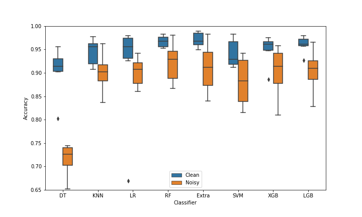
As Figure 2 shows, performance of all classifiers get worse, which is expected. But there is a pretty huge variation among classifiers. Decision Tree (DT) appears to be extremely vulnerable to noise. All 4 ensembles examined here: Random Forest (RF), Extra Tree (Extra), XGBoost (XGB) and LightGBM (LGB), have broadly similar performance on original data. But XGBoost’s performance takes a comparatively bigger hit due to noise, RF on the other hand seems comparatively robust.
How Exactly Label Noise Harms Performance
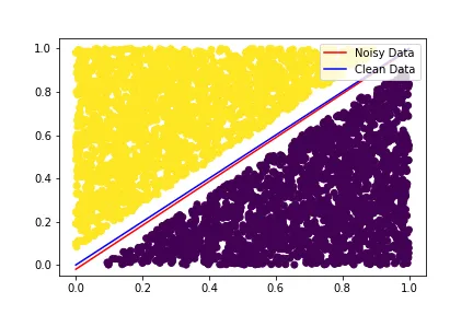
Well, an obvious answer is that low-quality data results in low-quality models. But defining quality isn’t straight as forward as it seems. We might be tempted to say dataset with higher noise level is of lower quality, and intuitively that makes sense. But remember figure 1? here is the same one, but now with 4000 samples instead of 400. In both cases the datasets contain 30% label noise, so should be of similar quality. Yet in this case, the decision boundary learned with noisy data is indistinguishable from the one learned with clean data. This isn’t to say that the intuition is wrong (it isn’t), but to emphasize that when it comes to explaining the performance loss, there’s more to the story (e.g. dataset size) than simple noise level.
Besides, the data-centric perspective alone doesn’t explain the huge disparity among different classifiers’ response to noise. So next we’re going to analyze it from the perspective of classifiers. In the figure below, we take the most brittle among all classifiers- Decision Tree, train it with both clean and noisy labels of Iris dataset, and plot the structure of resulting trees below.
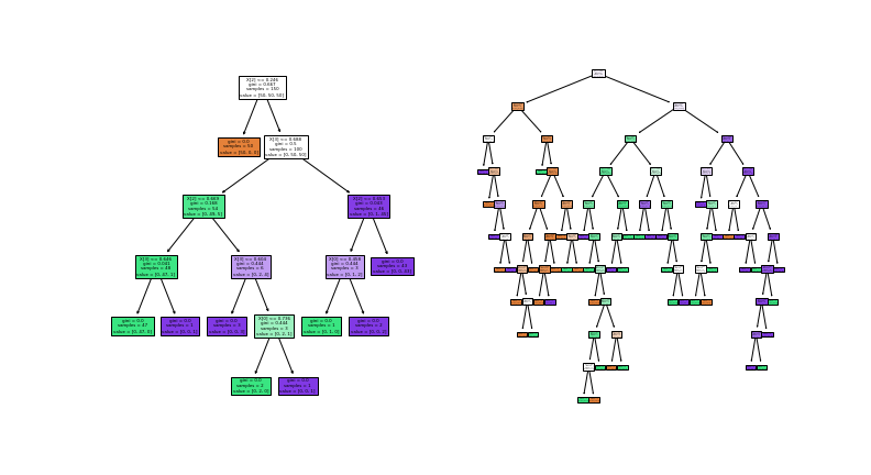
We’re only applying 20% noise here. But even this small noise is enough to turn a relatively small decision tree (left) into a gigantic mess (right). This is admittedly a contrived and extreme example, but it does reveal an important insight that more or less applies to all classifiers: label noise increases the model complexity, making the classifiers overfit to noise.
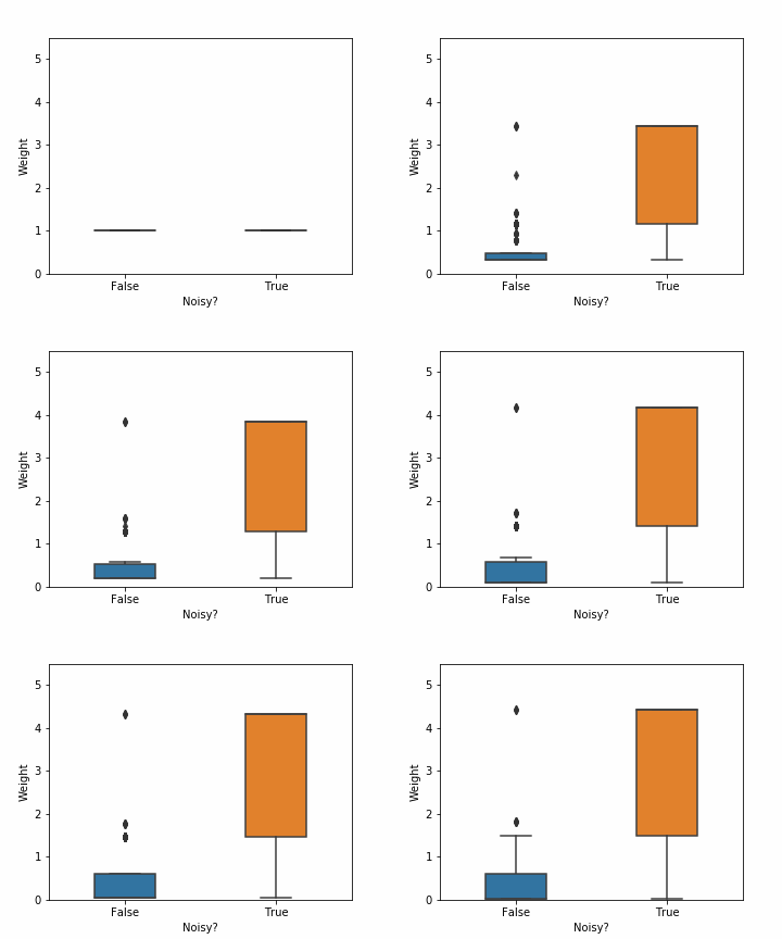
Another good algorithm to demonstrate the impact of noise is Adaboost, the predecessor of current state-of-the-arts like XGBoost and LightGBM. It was among state-of-the-arts in early 2000s, but it is also very vulnerable to label noise. Adaboost begins by assigning each instance equal weight. At each iteration, it increases the weight of the instances it misclassified, and reduces the weight of others. In this way, it gradually concentrates more on the harder instances. But as you might have imagined, mislabeled instances are usually harder to classify than clean ones. So Adaboost ends up assigning higher weights to mislabeled samples i.e. it tries hard to correctly classify instances it should ideally ignore. The animation in figure 5 captures the distribution of weights assigned to noisy and clean samples by Adaboost on Breast Cancer dataset with 20% noise. After only 20 iterations, noisy instances collectively have twice more weight than clean ones, despite being outnumbered 4 to 1.
To make this discussion complete, let’s take a look at some classifiers of the opposite spectrum: ones that are more robust to noise than others. If you have looked at figure 2 attentively, you’ve probably discovered a quite remarkable fact: that two of the most robust classifiers there (Random Forest and Extra Tree) are nothing but a simple collection of the most brittle algorithm: Decision Tree. To explain this, let’s start with something that these forests doesn’t do- they don’t put extra emphasis on noisy instances like Adaboost (or SVM), all instances are treated equally during bootstrap aggregating (or Bagging) [3], a vital component of random forest.
The explanation of how a bunch of poor decision trees (DT) can band together to form such powerful random forest lies in a concept called bias–variance decomposition of classification error. Imagine lots of DTs each with exactly 60% accuracy on a binary classification dataset. Assuming there is no correlation between their predictions, given a new instance, we can expect (approximately) 60% of DTs to make the right prediction on it. So if we aggregate their result by majority voting, for any new instance majority (i.e. 60%) will make the right prediction, giving us a perfect 100% accuracy! Of course, that assumption of zero correlation is impossible to achieve in practice, so we can’t go quite as far as 100, but hopefully, you get the point.
Handling Label Noise
Before we start talking about mitigating the impact of noise, please remember the famous No Free Lunch theorem. None of the methods discussed below are panacea- they sometimes work and sometimes don’t. And sometimes when they do work, the improvement might be insignificant compared to added computational cost. So always remember to compare your ML pipeline against a simple baseline without any of these noise handling mechanisms.
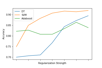
That being said, broadly speaking, we can attack the label noise problem from two angles: by using noise robust algorithms, or by cleaning our data. In the first approach, we can simply pick algorithms that are inherently more robust, for example, bagging-based ensembles over boosting. There have also been many algorithms and loss functions designed specifically to be noise-robust, for example unhinged SVM [4][5]. Or, using the fact that label noise leads to overfitting, we can usually make brittle algorithms more robust just by introducing stronger regularization, as figure 6 shows.
For cleaning data, we can use the previously stated observation that mislabeled instances are harder to correctly classify. In fact, a good number of ML papers rely on this observation to design new data cleaning procedures [6]. The basic steps are: train a bunch of classifiers using a subset of training data, predict the labels of the rest of the data using them, and then the percentage of classifiers that failed to correctly predict a sample’s given label is the probability that the sample is mislabeled. Although a link to full code has already been shared, a sample implementation using an ensemble of decision trees is so simple that I can’t resist showing it here:
def detect_noisy_samples(X,y,thres=.5): #Returns noisy indexes
    rf = RandomForestClassifier(oob_score=True).fit(X,y)
    noise_prob = 1 - rf.oob_decision_function_[range(len(y)),y]
    return noise_prob>thres
On Spambase dataset with 25% label noise, this method detects 85% of mislabeled instances, while only 13% of clean instances get detected as noisy. For Breast Cancer, these numbers are 90% and 10% respectively.
But this method of training multiple classifiers only to preprocess dataset might be impractical for big datasets. Another closely related but far more efficient heuristic is: 1) find the K nearest neighbors of a sample, 2) compute the percentage of those neighbors with similar label, 3) Use that as a proxy for label reliability. As expected, it’s performance can be somewhat less impressive- it detects 2/3rd of noisy instances in Spambase while 10% of clean instances gets labeled noisy. But once again, a basic implementation is incredibly simple.
def detect_noisy_samples(X,y,thres=.5): #Returns noisy indexes
    knn = KNeighborsClassifier().fit(X,y)
    noise_prob = 1 - knn.predict_proba(X)[range(len(X)),y]
    return np.argwhere(noise_prob>thres).reshape(-1)
It is worth emphasizing that cleaning data doesn’t have to mean simply throwing away suspected mislabeled samples. Both of the heuristics described above returns continuous probability of (a sample) being mislabeled. We can use the inverse of that probability as a sort of reliability or confidence score, and use cost-sensitive learning to utilize this information. In this way, we get to retain all data points, which is especially important when the noise level is high or dataset size is small. Plus, this is more general than filtering- filtering is a special instance of cost-sensitive approach where the cost can be only 0 and 1.
Conclusion
Thanks for staying this far! I hope this article has been useful. But please remember that this is simply an introduction, and therefore leaves out a lot of interesting and important questions.
For example, we haven’t really talked about “Noise Model” here. We only focused on the overall percentage of mislabeled samples, assuming the wrong label for a mislabeled instance can come from any of the other labels with equal probability. This is not unrealistic, this so-called uniform noise model can arise e.g. when an amazon bot randomly assigns labels. But we know from common sense that a serious human annotator is much more likely to confuse between say 9 and 7 than 9 and 8, or between positive and neutral sentiment than positive and negative sentiment- and the uniform noise model doesn’t quite capture this uneven interaction between labels.
Another interesting question is regarding how we should act when we haven’t yet collected labels: Do we collect a big amount of low-quality data? or do we collect a small quantity of high-quality data?
Anyway, I hope this introduction serves as a good starting point. I’m planning to address these left-out issues and several others in a series of articles in near future, so stay tuned.
References
[1] https://escholarship.org/uc/item/9zt9g3wt
[2] https://ieeexplore.ieee.org/document/8765743
[3] G., Yves. “Bagging equalizes influence.” Machine Learning, (2004)
[4] http://papers.nips.cc/paper/5941-learning-with-symmetric-label
[5] http://papers.nips.cc/paper/5073-learning-with-noisy-labels
[6] https://ieeexplore.ieee.org/abstract/document/6685834
Enjoy Reading This Article?
Here are some more articles you might like to read next: